Inverse Problems and Applications (06w5092)
Organizers
Gary Margrave (University of Calgary)
Gunther Uhlmann (University of Washington and HKUST)
Description
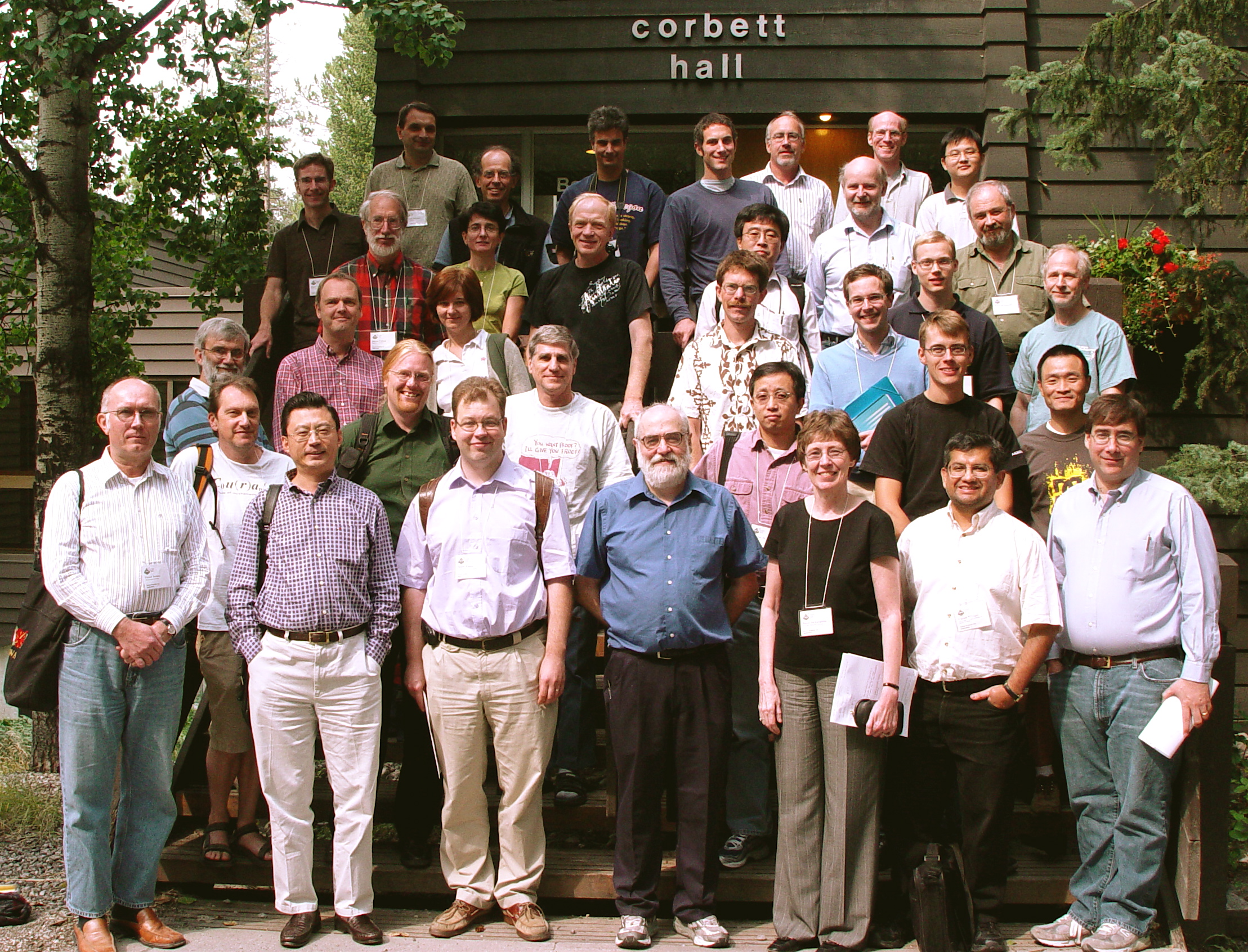
Some of the most high powered experts in the world will converge on The Banff Centre, August 19-24, 2006, where the Banff International Research Station will be hosting a workshop on recent developments in inverse problems. This event is co-organized by Professor Gary Margrave, a geophysicist at the University of Calgary and Professor Gunther Uhlmann, a mathematician at the University of Washington. The workshop will focus on the hottest new results in both theoretical and practical aspects of inverse problems. Inverse Problems are problems where causes for a desired or observed effect are to be determined and they arise in all fields of science and industry. The experts will discuss recent results on medical imaging techniques like elastography, electric impedance tomography, magnetic resonance imaging, optical tomography and thermoacoustic tomography among others. Other topics of discussion will be new imaging techniques used in oil exploration and remote sensing.
The Banff International Research Station for Mathematical Innovation and Discovery (BIRS) is a collaborative Canada-US-Mexico venture that provides an environment for creative interaction as well as the exchange of ideas, knowledge, and methods within the Mathematical Sciences, with related disciplines and with industry. The research station is located at The Banff Centre in Alberta and is administered by the Pacific Institute for the Mathematical Sciences, in collaboration with the Mathematics of Information Technology and Complex Systems Network (MITACS), the Berkeley-based Mathematical Science Research Institute (MSRI) and the Instituto de Matematicas at the Universidad Nacional Autonoma de Mexico (UNAM).
The Banff International Research Station for Mathematical Innovation and Discovery (BIRS) is a collaborative Canada-US-Mexico venture that provides an environment for creative interaction as well as the exchange of ideas, knowledge, and methods within the Mathematical Sciences, with related disciplines and with industry. The research station is located at The Banff Centre in Alberta and is administered by the Pacific Institute for the Mathematical Sciences, in collaboration with the Mathematics of Information Technology and Complex Systems Network (MITACS), the Berkeley-based Mathematical Science Research Institute (MSRI) and the Instituto de Matematicas at the Universidad Nacional Autonoma de Mexico (UNAM).